Code
#load libraries
library(tidyverse)
library(gt)
library(ggrepel)#load libraries
library(tidyverse)
library(gt)
library(ggrepel)It’s an exciting time for volleyball in the United States. The sport has been improving rapidly for the last 10-15 years, especially on the offensive side of the equation. Players are more athletic, dynamic and better trained coming into college. As a result, teams can push the boundaries of creativity in offensive schemes. But what teams are improving their offenses? Are there decent, but not great, offensive teams that still win a lot of games? Let’s explore.
First of all, I make no secret that I’m a Nebraska and Big Ten fan. So, to begin this exploration I’ll be looking at Nebraska and the Big Ten conference. However, my analysis will expand to the rest of the country (with comparisons to Nebraska made along the way).
To begin, let’s look at how Big Ten offenses fared between 2022 and 2023. This first chart simply displays the change in season hitting percentages from each Big Ten member between the 2022 and 2023 seasons. And if you’re not quite sure what a hitting percentage in volleyball is, it’s an efficiency that’s calculated by taking (your kills- your errors)/your total attempts.
#load in the data
offense <- read_csv("data/derek_offense.csv")

#make a slope chart for 2022 and 2023 offenses
#first make some vectors to be used later on
big_ten <- c("Nebraska","Wisconsin","Penn St.", "Michigan", "Michigan St.", "Iowa", "Purdue", "Illinois", "Minnesota", "Ohio St.", "Maryland", "Rutgers", "Northwestern", "Indiana")

big_ten_offense <- offense |>
  group_by(team_name, season)|>
  filter(team_name %in% big_ten)|>
  summarise(
    totalkills=sum(kills),
    totalerrors=sum(attack_errors),
    totalattempts=sum(attacks)
  )|>
  mutate(
    hit_pct=(totalkills-totalerrors)/totalattempts
  )|>
  select(
    team_name, hit_pct, season
  )

  nu <- big_ten_offense |> filter(team_name=="Nebraska")
  wis <- big_ten_offense |> filter(team_name=="Wisconsin")
  ind <- big_ten_offense |> filter(team_name=="Indiana")
  mich <- big_ten_offense |> filter (team_name=="Michigan")
  ggplot() +
  geom_line(
    data = big_ten_offense,
    aes(
      x = season,
      y = hit_pct,
      group = team_name
    ),
    color="grey")+
  geom_point(
    data = big_ten_offense,
    aes(
      x = season,
      y = hit_pct,
      group = team_name
    ),
    color="grey"
  )+
    geom_line(
    data = nu,
    aes(
      x = season,
      y = hit_pct,
      group = team_name
    ),
    color="black")+
  geom_point(
    data = nu,
    aes(
      x = season,
      y = hit_pct,
      group = team_name
    ),
    color="black"
  )+
    geom_line(
    data = wis,
    aes(
      x = season,
      y = hit_pct,
      group = team_name
    ),
    color="#C5050C")+
  geom_point(
    data = wis,
    aes(
      x = season,
      y = hit_pct,
      group = team_name
    ),
    color="#C5050C"
  )+
    geom_line(
    data = ind,
    aes(
      x = season,
      y = hit_pct,
      group = team_name
    ),
    color="#990000")+
  geom_point(
    data = ind,
    aes(
      x = season,
      y = hit_pct,
      group = team_name
    ),
    color="#990000"
  )+
    geom_line(
    data = mich,
    aes(
      x = season,
      y = hit_pct,
      group = team_name
    ),
    color="#00274c")+
  geom_point(
    data = mich,
    aes(
      x = season,
      y = hit_pct,
      group = team_name
    ),
    color="#00274c"
  )+
  scale_x_continuous(
    breaks=c(2022, 2023),
    limits=c(2021.75, 2023.25)
  ) +
    scale_y_continuous(
      breaks=c(.175, .200, .225, .250, .275, .300, .325)
    )+
  geom_text(
    data = nu |> filter(season == max(season)),
    aes(
      x = season + .1,
      y = hit_pct ,
      group = team_name,
      label = team_name
    ))+
  geom_text(
    data = nu |> filter(season == min(season)),
    aes(
      x = season - .1,
      y = hit_pct,
      group = team_name,
      label = team_name
    ))+
  geom_text(
    data = wis |> filter(season == max(season)),
    aes(
      x = season + .1,
      y = hit_pct ,
      group = team_name,
      label = team_name
    ))+
  geom_text(
    data = wis |> filter(season == min(season)),
    aes(
      x = season - .1,
      y = hit_pct,
      group = team_name,
      label = team_name
    ))+
  geom_text(
    data = ind |> filter(season == max(season)),
    aes(
      x = season + .1,
      y = hit_pct ,
      group = team_name,
      label = team_name
    ))+
  geom_text(
    data = ind |> filter(season == min(season)),
    aes(
      x = season - .1,
      y = hit_pct,
      group = team_name,
      label = team_name
    ))+
  geom_text(
    data = mich |> filter(season == max(season)),
    aes(
      x = season + .1,
      y = hit_pct ,
      group = team_name,
      label = team_name
    ))+
  geom_text(
    data = mich |> filter(season == min(season)),
    aes(
      x = season - .1,
      y = hit_pct,
      group = team_name,
      label = team_name
    ))+
    theme_minimal()+
  labs(
    x= "Season",
    y = "Hitting Percentage",
    title = "Wisconsin continues to dominate offensively in Big Ten",
    subtitle = "Michigan had a bad year one after coaching change",
    caption="Data courtesy of Evollve.net | By Derek Harrington"
  ) +
  theme(
    plot.title = element_text(size = 16, face = "bold"),
    plot.subtitle = element_text(size = 12),
    axis.title = element_text(size = 10),
    panel.grid.minor = element_blank(),
    plot.title.position = "plot"
  )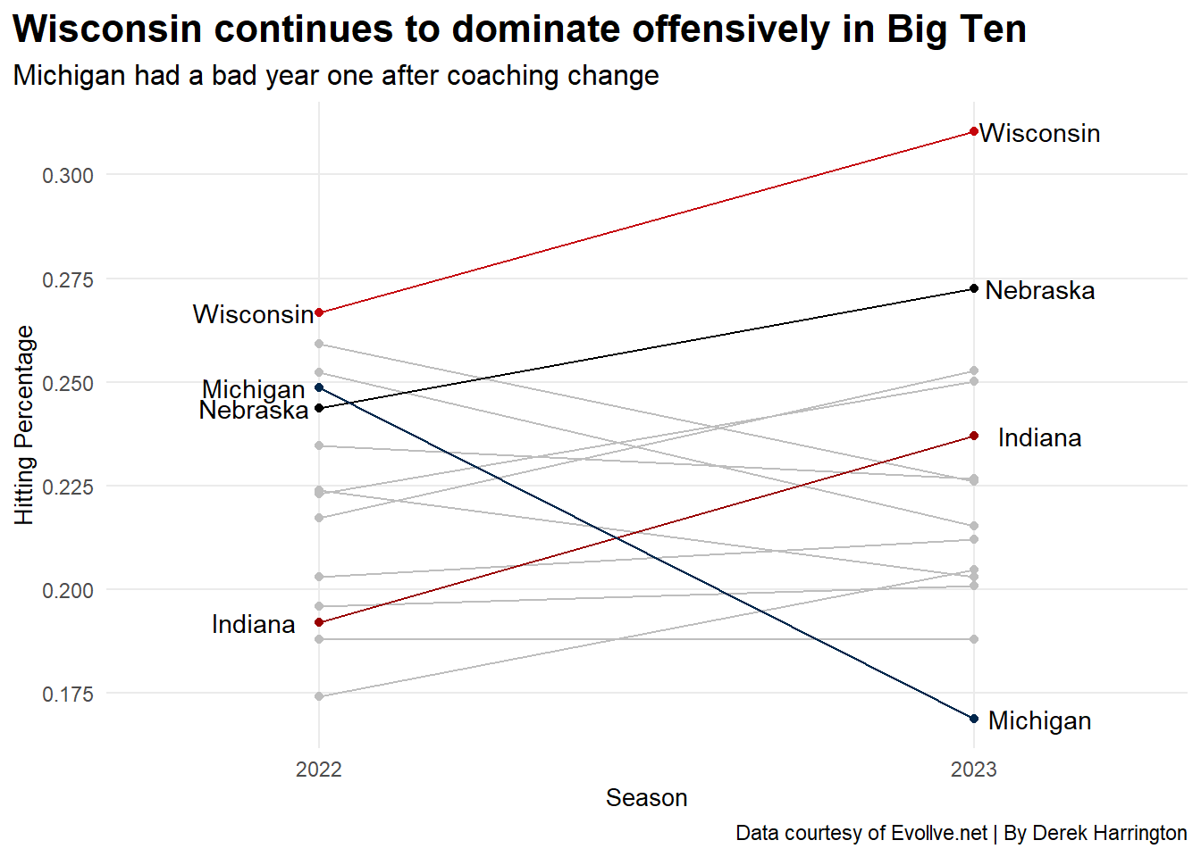
So, what to make of this? Well, first of all, Wisconsin was the national champion in 2021. They lost many key pieces from that team including Dana Rettke and Sydney Hilley. And yet, they were still atop the Big Ten in 2022 in terms of hitting percentage, and to no one’s surprise, they won the conference title. The Huskers switched to a 6-2 offense in 2022 and the offensive numbers were up from 2021. If not for a crippling injury in the last week of the regular season that forced some lineup changes, Nebraska may have been able to win the conference title. But I digress. The interesting story comes in 2023 in my opinion.
As the chart shows, Wisconsin improved its offense from 2022 to 2023, hitting over .300 as a team! The Badgers were no doubt among the elite offensive teams across the country. We can also see that Nebraska made a sizable jump, thanks to newcomers that included Merritt Beason, Harper Murray, Andi Jackson and Bergen Reilly (among many other important pieces). This chart would suggest that Wisconsin still ran away with the conference title as there’s a sizable gap between the Huskers and Badgers offensively.
But….Nebraska actually won the conference title. Nebraska was the nation’s best defensive team last year, and that paired with the offensive improvement led to the Huskers claiming the Big Ten title outright. It’s also only fair to point out that Wisconsin had a couple of injuries toward the end of the year that allowed Purdue and Penn State to knock off the Badgers, allowing the Huskers to claim the title. Nevertheless, it’s a prime example of offense not always being the main story. So, if Nebraska won the conference in 2023 and had a chance to win it in 2022, but it wasn’t close to touching Wisconsin in team hitting percentage,so there’s something else there, but what?
Also note that Indiana made a huge improvement with its offense, which put the Hoosiers in contention for an at-large bid to the NCAA tournament. Unfortunately, the Hoosiers dropped some games early in the non-conference and late in the season that kept them out. Michigan had a rough year with a coaching change and roster turnover. However, if you were to compare the Wolverines’ 2023 numbers to those of 2024, you’d see a big improvement.
So, let’s take this examination up a level and look at the 2022 and 2023 seasons in a different light. Let’s examine the top 10 (using the end-of-year top 10 rankings) for each year and see how they fared with points earned and points given up.
In the most simplistic terms, the points per set a team earns is the addition of the kills per set, aces per set and blocks per set. Typically, you’d want to be in the range of 17 to 18 earned points per set to be considered elite. Points given up is the summation of all of your errors (hitting, serving, ball handling and block errors). Obviously with points given up you want to be as low as possible. So, let’s take a look for both 2022 and 2023.
#|message: FALSE

#make some more vectors with teams from the power 5 conferences

sec <- c("Florida", "Kentucky", "Missouri", "Alabama", "Arkansas", "Georgia", "Ole Miss", "Miss St.", "Tennessee", "South Carolina", "LSU", "Texas A&M", "Auburn")
pac_12 <- c("Stanford", "Oregon", "UCLA", "USC", "Arizona", "Arizona St.", "Colorado", "Utah", "Oregon St.", "Washington", "Washington St.", "California")
big_12_22 <- c("Texas", "Iowa St.", "Kansas", "Kansas St.", "Baylor", "Oklahoma", "TCU", "Texas Tech", "West Virginia")
big_12_23 <- c("Texas", "Iowa St.", "Kansas", "Kansas St.", "Baylor", "Oklahoma", "TCU", "Texas Tech", "Weest Virginia", "BYU", "UCF", "Houston", "Cincinnati")
acc <- c("Pittsburgh", "Florida St.", "Miami", "Clemson", "NC State", "Boston College", "Louisville", "Notre Dame", "Syracuse", "Duke", "North Carolina", "Wake Forest", "Georgia Tech", "Virginia", "Virginia Tech" )

power5_22 <- c(big_ten, sec, pac_12,big_12_22, acc)
power5_23 <- c(big_ten, sec, pac_12,big_12_23, acc)

top_ten22 <- c("Texas", "Louisville", "San Diego", "Pittsburgh", "Wisconsin", "Stanford", "Oregon", "Ohio St.", "Nebraska", "Minnesota")

top_ten23 <- c("Texas", "Nebraska", "Wisconsin", "Pittsburgh", "Stanford", "Louisville", "Oregon", "Arkansas", "Tennessee", "Kentucky")

offense_earned_given_22 <- offense |>

   select(
    team_name,
    season,
    aces,
    kills,
    sets_won,
    sets_lost,
    block_solos,
    block_assists,
    block_errors,
    service_errors,
    attack_errors,
    ball_handling_errors
  ) |>
  filter(season=="2022")|>
  group_by(team_name) |>
  drop_na()|>
  summarize(
    total_sets = sum(sets_won+ sets_lost),
    earned_pts = sum(aces + kills +(block_solos + (block_assists/2))),
    pts_given = sum(service_errors + attack_errors +block_errors+ball_handling_errors)
  ) |>
  mutate(
    earned_pts_set = earned_pts/total_sets,
    given_pts_set= pts_given/total_sets

  ) |>
  rename(Team = team_name) |>
  select(Team, earned_pts_set, given_pts_set) |>
  filter(Team %in% top_ten22)|>
  arrange(desc(earned_pts_set))

offense_earned_given_23 <- offense |>

   select(
    team_name,
    season,
    aces,
    kills,
    sets_won,
    sets_lost,
    block_solos,
    block_assists,
    block_errors,
    service_errors,
    attack_errors,
    ball_handling_errors
  ) |>
  filter(season=="2023")|>
  group_by(team_name) |>
  drop_na()|>
  summarize(
    total_sets = sum(sets_won+ sets_lost),
    earned_pts = sum(aces + kills +(block_solos + (block_assists/2))),
    pts_given = sum(service_errors + attack_errors +block_errors+ball_handling_errors)
  ) |>
  mutate(
    earned_pts_set = earned_pts/total_sets,
    given_pts_set= pts_given/total_sets

  ) |>
  rename(Team = team_name) |>
  select(Team, earned_pts_set, given_pts_set) |>
  filter(Team %in% top_ten23)|>
  arrange(desc(earned_pts_set))


#make a table for 22 pts/earned per set

 offense_earned_given_22 |>
  gt()|>
  cols_label(
    earned_pts_set="Earned Pts/set",
    given_pts_set="Errors/set"
  )|>
  tab_header(
    title = "Stanford had no problems scoring against teams in 2022",
    subtitle = "Texas didn't gift many points"
  )|>
   tab_style(
    style = cell_text(color = "black", weight = "bold", align = "left"),
    locations = cells_title("title")
  ) |>
  tab_style(
    style = cell_text(color = "black", align = "left"),
    locations = cells_title("subtitle")
  )|>
  tab_source_note(
    source_note = md("By **Derek Harrington**  <br>Data courtesy of **Evollve.net**"))|>
   tab_style(
    locations = cells_column_labels(columns = everything()),
    style = list(
      cell_borders(sides = "bottom", weight = px(3)),
      cell_text(weight = "bold", size = 12)))|>
    opt_row_striping() |>
  opt_table_lines("none") |>
  fmt_number(
    columns = c(earned_pts_set, given_pts_set),
    decimals = 2)|>
  tab_style(
    style = list(
      cell_fill(color = "white"),
      cell_text(color = "darkgreen", weight="bold")
    ),
    locations = cells_body(
      rows = Team == "Texas"
    ))|>
      tab_style(
    style = list(
      cell_fill(color = "white"),
      cell_text(color = "red", weight="bold")
    ),
    locations = cells_body(
      rows = Team == "Nebraska"

))| Stanford had no problems scoring against teams in 2022 | ||
|---|---|---|
| Texas didn't gift many points | ||
| Team | Earned Pts/set | Errors/set |
| Stanford | 18.84 | 7.79 |
| Texas | 18.68 | 6.50 |
| Wisconsin | 18.00 | 7.16 |
| San Diego | 17.87 | 6.79 |
| Pittsburgh | 17.72 | 7.06 |
| Louisville | 17.66 | 7.20 |
| Ohio St. | 17.46 | 7.64 |
| Minnesota | 17.40 | 6.77 |
| Oregon | 17.30 | 7.29 |
| Nebraska | 16.63 | 7.76 |
| By Derek Harrington Data courtesy of Evollve.net |
||
What’s the story here? First of all, the thing jumping off the page to me is Stanford was earning nearly 19 points a set which is truly outstanding. However, they also led the top 10 in points given away per set. Perhaps that’s one of the reasons why San Diego was able to upset the Cardinal in the regional final at Stanford. Both teams were tremendous in 2022, but on average, San Diego didn’t give away as many points as Stanford.
Texas ranks second for total points earned per set and that’s not a surprise. That Texas team had Logan Eggleston, Madi Skinner and Asjia O’Neal as its go-to hitters. They were truly a great offensive team AND they also didn’t gift you many free points. If you lined up against the Longhorns, you were going to have to earn every point.
Nebraska ranks last for earned points per set, which is a bit surprising considering the 6-2 had improved its offense over 2022. The final numbers may have been impacted somewhat by the changes in personnel due to the injury, but I’m not sure it would make that big of a difference. The 2022 Huskers were also giving away far too many points to other teams, ranking second just behind Stanford.
So, recalling Nebraska’s offensive jump from 2022 to 2023, did the Huskers make a significant jump in the 2023 standings?
 offense_earned_given_23 |>
  gt()|>
   cols_label(
    earned_pts_set="Earned Pts/set",
    given_pts_set="Errors/set"
  )|>
     tab_header(
    title = "Stanford continued its dominance over the field in 2023",
    subtitle = "Nebraska earned more points, but Texas still won the title"
  )|>
   tab_style(
    style = cell_text(color = "black", weight = "bold", align = "left"),
    locations = cells_title("title")
  ) |>
  tab_style(
    style = cell_text(color = "black", align = "left"),
    locations = cells_title("subtitle")
  )|>
  tab_source_note(
    source_note = md("By **Derek Harrington**  <br>Data courtesy of **Evollve.net**"))|>
   tab_style(
    locations = cells_column_labels(columns = everything()),
    style = list(
      cell_borders(sides = "bottom", weight = px(3)),
      cell_text(weight = "bold", size = 12)))|>
    opt_row_striping() |>
  opt_table_lines("none") |>
  fmt_number(
    columns = c(earned_pts_set, given_pts_set),
    decimals = 2)|>
  tab_style(
    style = list(
      cell_fill(color = "white"),
      cell_text(color = "darkgreen", weight="bold")
    ),
    locations = cells_body(
      rows = Team == "Texas"
    )
  )|>
   tab_style(
    style = list(
      cell_fill(color = "white"),
      cell_text(color = "red", weight="bold")
    ),
    locations = cells_body(
      rows = Team == "Nebraska"
))| Stanford continued its dominance over the field in 2023 | ||
|---|---|---|
| Nebraska earned more points, but Texas still won the title | ||
| Team | Earned Pts/set | Errors/set |
| Stanford | 19.02 | 7.88 |
| Tennessee | 18.71 | 7.19 |
| Wisconsin | 18.52 | 6.42 |
| Oregon | 18.29 | 7.58 |
| Pittsburgh | 18.19 | 6.95 |
| Texas | 17.92 | 6.84 |
| Kentucky | 17.80 | 7.79 |
| Arkansas | 17.74 | 7.28 |
| Nebraska | 17.73 | 7.95 |
| Louisville | 17.64 | 7.44 |
| By Derek Harrington Data courtesy of Evollve.net |
||
Nope. Sure, Nebraska did improve slightly in total earned points per set, getting into the upper 17s, but there were clearly teams better at earning points than the Huskers. the Stanford did eclipse the 19 earned points per set mark in 2023. However, the Cardinal lost yet again in the regional final, at home, this time to the Texas Longhorns. Stanford losing at home in the regional final in back-to-back years, especially with how dominate they were, is quite thought-provoking.
Nebraska only slightly improved its earned points per set, and it led the top 10 teams in errors per set. And yet, the Huskers made it to the national championship and only lost two games. Texas, who knocked off Stanford, Wisconsin and Nebraska en route to the title, put together a remarkable post-season run. It’s more impressive when you consider the fact Texas faced match point in the fourth set against Tennessee in the regional semifinal. But the Longhorns prevailed over the Volunteers and weren’t seriously challenged the rest of the tournament.
So, there’s an element that’s still missing here. Why was Nebraska the team to beat in 2023 even though the above numbers suggest they were only slightly better than in 2022? Well….if you followed social media whenever Nebraska played in 2023 there was a common theme. It would be pointed out that it seemed teams couldn’t keep a serve in play to save their lives when they faced Nebraska. But is that really what happened?
#make a table showing opponents errors for 2023
#make new dataframe for Nebraska's gifts
Nebraska_gifted23 <- offense |>
  filter(season=="2023")|>

   select(
    team_name,
    aces,
    kills,
    sets_won,
    sets_lost,
    block_solos,
    block_assists,
    block_errors,
    service_errors,
    attack_errors,
    ball_handling_errors,
    opp_service_errors,
    opp_attack_errors,
    opp_ball_handling_errors
  ) |>
  group_by(team_name) |>
  drop_na()|>
  summarize(
    total_sets = sum(sets_won+ sets_lost),
    earned_pts = sum(aces + kills +(block_solos + (block_assists/2))),
    pts_given = sum(service_errors + attack_errors +block_errors+ball_handling_errors),
    gift_points= sum(opp_service_errors + opp_ball_handling_errors + opp_attack_errors),
    se_gifts=sum(opp_service_errors)
  ) |>
  mutate(
    earned_pts_set = earned_pts/total_sets,
    given_pts_set= pts_given/total_sets,
    unearned_pts_set=gift_points/total_sets,
    SE=se_gifts

  ) |>
  rename(Team = team_name) |>
  select(Team, unearned_pts_set,SE) |>
  filter(Team %in% top_ten23)|>
  arrange(desc(SE))


#table with service errors from opponents

Nebraska_gifted23 |>
  gt(
  )|>
  cols_label(
    SE="Opp service errors",
    unearned_pts_set="Opp errors/set"
  )|>
     tab_header(
    title = "Nebraska's opponents were error-prone",
    subtitle = "Huskers' opponents served too aggressively"
  )|>
   tab_style(
    style = cell_text(color = "black", weight = "bold", align = "left"),
    locations = cells_title("title")
  ) |>
  tab_style(
    style = cell_text(color = "black", align = "left"),
    locations = cells_title("subtitle")
  )|>
  tab_source_note(
    source_note = md("By **Derek Harrington**  <br>Data courtesy of **Evollve.net**"))|>
   tab_style(
    locations = cells_column_labels(columns = everything()),
    style = list(
      cell_borders(sides = "bottom", weight = px(3)),
      cell_text(weight = "bold", size = 12)))|>
    opt_row_striping() |>
  opt_table_lines("none") |>
  fmt_number(
    columns = c(Team, SE),
    decimals = 0)|>
  tab_style(
    style = list(
      cell_fill(color = "white"),
      cell_text(color = "darkgreen", weight="bold")
    ),
    locations = cells_body(
      rows = Team == "Nebraska"
    )
)| Nebraska's opponents were error-prone | ||
|---|---|---|
| Huskers' opponents served too aggressively | ||
| Team | Opp errors/set | Opp service errors |
| Nebraska | 8.735537 | 325 |
| Texas | 8.551402 | 277 |
| Stanford | 7.300000 | 269 |
| Arkansas | 7.401575 | 265 |
| Louisville | 7.948718 | 260 |
| Oregon | 7.928571 | 260 |
| Pittsburgh | 8.387931 | 260 |
| Kentucky | 6.916667 | 230 |
| Wisconsin | 8.260504 | 227 |
| Tennessee | 7.226415 | 222 |
| By Derek Harrington Data courtesy of Evollve.net |
||
Yes! Whoever played Nebraska seemed to have issues with keeping the ball in play. Not only did the Huskers lead the top 10 in points gifted by the other team, but they also led in opponent service errors. The question on your mind is probably why? A logical guess would be that because Nebraska was such a good passing team in 2023 AND the Huskers had some formidable attackers, teams had to crank up the service pressure to get them out-of-system.
The downside to that is the amount of service errors. This makes Texas’ win in the national championship even more impressive because they served Nebraska off the court and perhaps, Nebraska didn’t know what to do when they weren’t getting the free points they were accustomed to. By all accounts, Nebraska is an even better passing team in 2024 so it would be interesting to revisit these numbers to see if there’s a similar story in 2024.
Perhaps the best metric to look at is hitting differential, which is your hitting efficiency minus your opponent’s hitting efficiency. Hitting differentials can be examined in a couple of different ways. Let’s look at the top 10 teams in 2023 and their hitting differentials.
#make dataframe for hitting differential
hitting_differential_23 <- offense |>

   select(
    team_name,
    season,
    kills,
   attack_errors,
   opp_kills,
   opp_attack_errors,
   attacks,
   opp_attacks

  ) |>
  filter(season=="2023")|>
  group_by(team_name) |>
  drop_na()|>
  summarize(
    total_kills = sum(kills),
    total_errors = sum(attack_errors),
    total_attempts = sum(attacks),
    total_opp_kills = sum(opp_kills),
    total_opp_errors = sum(opp_attack_errors),
    total_opp_attacks = sum(opp_attacks)
  ) |>
  mutate(
   hitting_pct = (total_kills - total_errors)/total_attempts,
   opponent_hit_pct = (total_opp_kills - total_opp_errors)/total_opp_attacks,
   hit_dif = hitting_pct - opponent_hit_pct


  ) |>
  rename(Team = team_name) |>
  select(Team, hit_dif) |>
  filter(Team %in% top_ten23)|>
arrange(desc(hit_dif))nu <- hitting_differential_23 |> filter (Team=="Nebraska")
tex <- hitting_differential_23 |> filter (Team=="Texas")
Wis <- hitting_differential_23 |> filter (Team=="Wisconsin")
Pitt <- hitting_differential_23 |> filter (Team=="Pittsburgh")
ggplot() +
geom_bar(
data = hitting_differential_23,
aes(
x = reorder(Team, hit_dif),
weight = hit_dif,
alpha = .3
)
) +
geom_bar(
data = nu,
aes(
x = reorder(Team, hit_dif),
weight = hit_dif),
fill = "red"
) +
geom_bar(
data = tex,
aes(
x = reorder(Team, hit_dif),
weight = hit_dif),
fill="red"
)+
geom_bar(
data =Wis,
aes(
x = reorder(Team, hit_dif),
weight = hit_dif),
fill="red")+
geom_bar(
data = Pitt,
aes(
x = reorder(Team, hit_dif),
weight = hit_dif),
fill="red")+
coord_flip() +
labs(
title = "Hitting differential more accurate predictor of 2023 Final Four teams",
subtitle= "Pitt and Nebraska made up for offense with defense",
x = "Team",
y = "Hitting Diferential",
caption="Data Courtesy of Evollve.net | By Derek Harrington")+
theme_minimal() +
theme(
plot.title = element_text(size = 15, face = "bold"),
plot.subtitle = element_text(size = 12),
axis.title = element_text(size = 10),
panel.grid.minor = element_blank(),
plot.title.position = "plot",
legend.position="none"
) 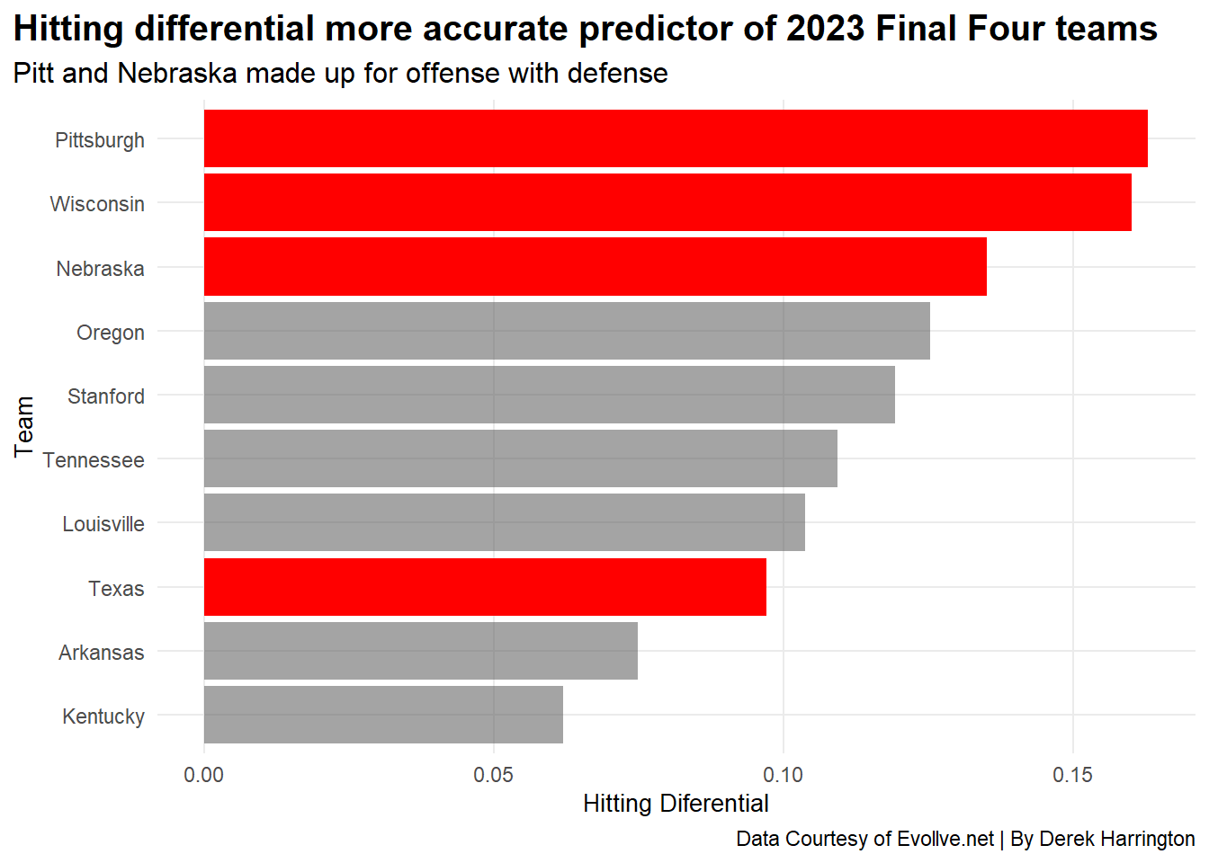
As we can see, three of the top four teams that led the country in hitting differential made the 2023 Final Four. Oregon, who sat fourth, lost to Wisconsin in a regional final. Stanford, Tennessee and Texas were all in the same regional. It’s clear that hitting differential can give you a pretty accurate idea of what teams could be considered favorites in the post season.
But these hitting differentials don’t necessarily mean the same thing for each team. Remember, Wisconsin was hitting above .300 as a team last year, but they’re second in hitting differential, meaning teams could score against the badgers. Conversely, for Pitt and Nebraska, while they both had a modest hitting efficiency, they held two of the top three spots indicating they had suffocating defenses.
One last interesting thing to look at is how these hitting differentials evolve over the course of a season. Let’s look at a step chart for both the 2022 and 2023 seasons.
hit_def_step_22 <- offense |>

   select(
    team_name,
    season,
    game_date,
    kills,
   attack_errors,
   opp_kills,
   opp_attack_errors,
   attacks,
   opp_attacks

  ) |>
  filter(season=="2022")|>
  drop_na()|>
   group_by(team_name, game_date)|>
  summarize(
    total_kills = sum(kills),
    total_errors = sum(attack_errors),
    total_attempts = sum(attacks),
    total_opp_kills = sum(opp_kills),
    total_opp_errors = sum(opp_attack_errors),
    total_opp_attacks = sum(opp_attacks)
  ) |>
 mutate(
   Cumkills = cumsum(total_kills),
   Cumattacks= cumsum(total_attempts),
   Cumerrors = cumsum(total_errors),
   Cumoppkills=cumsum(total_opp_kills),
   Cumopperrors=cumsum(total_opp_errors),
   Cumoppattacks=cumsum(total_opp_attacks),
   Cumhitpct = (Cumkills -  Cumerrors)/Cumattacks,
   Cumopp_hitpct = (Cumoppkills -Cumopperrors)/Cumoppattacks,
   Cumhit_dif = Cumhitpct - Cumopp_hitpct
   )|>


  rename(Team = team_name) |>
  select(Team,game_date, Cumkills, Cumattacks, Cumerrors, Cumoppkills,Cumopperrors, Cumoppattacks, Cumhit_dif) |>
  filter(Team %in% top_ten22)


#dataframe for 2023 hitting difference
hit_def_step_23 <- offense |>

   select(
    team_name,
    season,
    game_date,
    kills,
   attack_errors,
   opp_kills,
   opp_attack_errors,
   attacks,
   opp_attacks

  ) |>
  filter(season=="2023")|>
  drop_na()|>
   group_by(team_name, game_date)|>
  summarize(
    total_kills = sum(kills),
    total_errors = sum(attack_errors),
    total_attempts = sum(attacks),
    total_opp_kills = sum(opp_kills),
    total_opp_errors = sum(opp_attack_errors),
    total_opp_attacks = sum(opp_attacks)
  ) |>
 mutate(
   Cumkills = cumsum(total_kills),
   Cumattacks= cumsum(total_attempts),
   Cumerrors = cumsum(total_errors),
   Cumoppkills=cumsum(total_opp_kills),
   Cumopperrors=cumsum(total_opp_errors),
   Cumoppattacks=cumsum(total_opp_attacks),
   Cumhitpct = (Cumkills -  Cumerrors)/Cumattacks,
   Cumopp_hitpct = (Cumoppkills -Cumopperrors)/Cumoppattacks,
   Cumhit_dif = Cumhitpct - Cumopp_hitpct
   )|>


  rename(Team = team_name) |>
  select(Team,game_date, Cumkills, Cumattacks, Cumerrors, Cumoppkills,Cumopperrors, Cumoppattacks, Cumhit_dif) |>
  filter(Team %in% top_ten23)

#make a step chart for 2022 and 2023 for hit diff


nu22 <- hit_def_step_22 |> filter(Team=="Nebraska")
ut22 <- hit_def_step_22 |> filter(Team=="Texas")
ggplot() +
  geom_step(
    data =hit_def_step_22 ,
    aes(x = game_date, y = Cumhit_dif, group = Team), color="grey")+
    geom_step(
    data =nu22 ,
    aes(x = game_date, y = Cumhit_dif, group = Team), color="#d00000"
      )+
   geom_step(
    data =ut22 ,
    aes(x = game_date, y = Cumhit_dif, group = Team), color="#bf5700"
      ) +
  scale_y_continuous(
      breaks=c(-.5, -.4, -.3,-.2, -.1, 0, .1, .2, .3)
    )+
  annotate(
    "text",
    x = (as.Date("2022-12-14")),
    y = .130,
    label = "Nebraska"
  ) +
  annotate(
    "text",
    x = (as.Date("2022-12-17")),
    y = .200,
    label = "Texas"
  ) +
  labs(
    x = "Date",
    y = "Hitting Differential",
    title = "Texas dominated both offensively and defensively in 2022",
    subtitle="Nebraska was about middle of the pack",
    caption="Data Courtesy of Evollve.net | By Derek Harrington") +
  theme_minimal() +
  theme(
    plot.title = element_text(
      size = 16, face = "bold"
    ),
    plot.subtitle = element_text(size = 12),
    axis.title = element_text(size = 10),
    panel.grid.minor = element_blank(),
    plot.title.position = "plot"
  )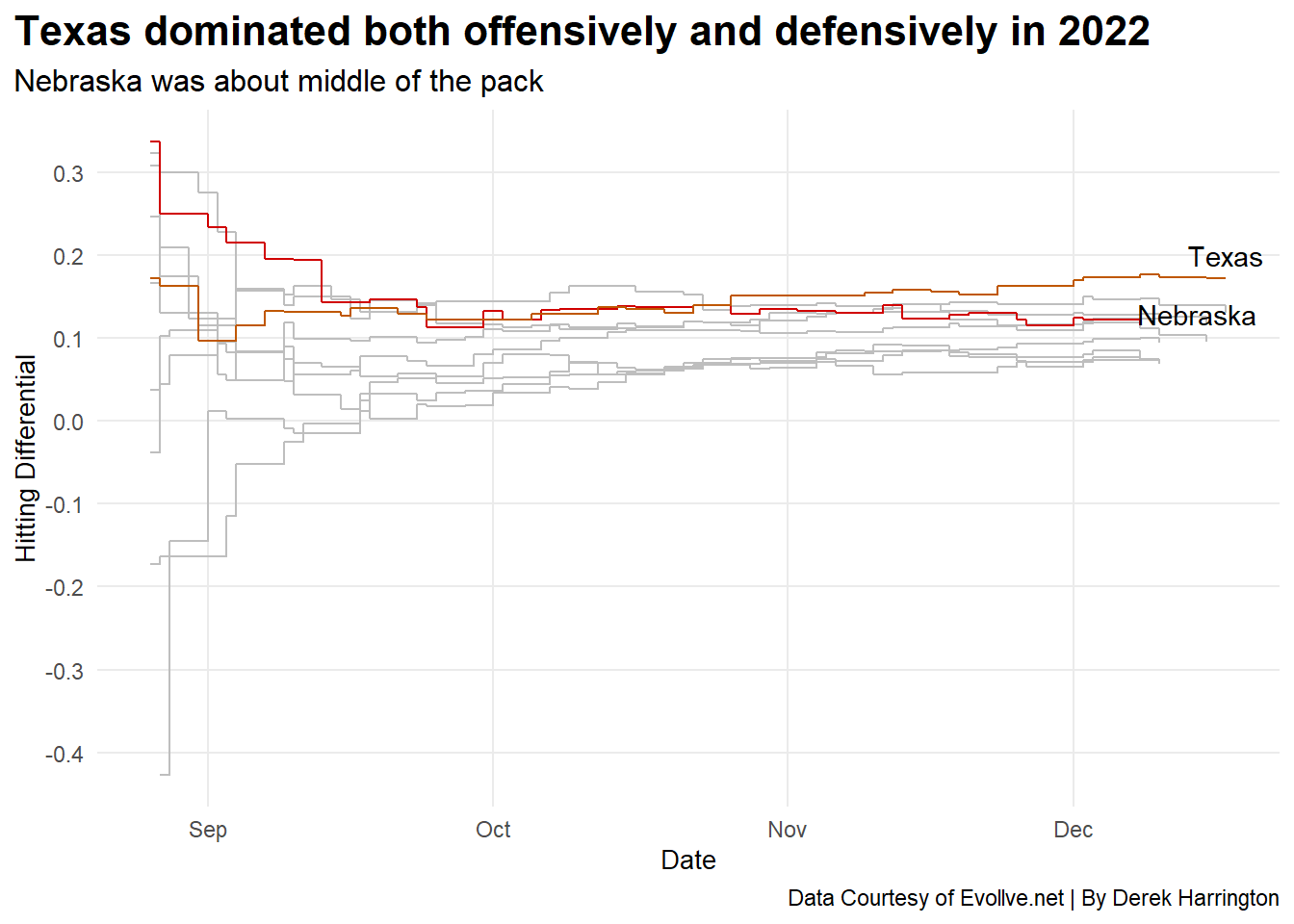
Texas started in the upper echelon of hitting differential in 2022, but not at the top. The brutal non-conference schedule that Texas had no doubt contributed to this. But, as Texas entered its Big 12 conference slate, its hitting differential continued to rise through the end of the year, and they led the country in that statistic after winning the championship match. Nebraska, on the flip side, started as the top team in this statistic but gradually fell through the beginning portions of the schedule and then leveled off once it got into Big Ten play. You can even see the dip right before December when the injury to Kenzie Knuckles occurred and lineup changes were made.
The 2023 season, however, tells a very different story.
nu23 <- hit_def_step_23 |> filter(Team=="Nebraska")
ut23 <- hit_def_step_23 |> filter(Team=="Texas")
ggplot() +
  geom_step(
    data =hit_def_step_23 ,
    aes(x = game_date, y = Cumhit_dif, group = Team), color="grey")+
   geom_step(
    data =nu23 ,
    aes(x = game_date, y = Cumhit_dif, group = Team), color="#d00000"
      )+
   geom_step(
    data =ut23 ,
    aes(x = game_date, y = Cumhit_dif, group = Team), color="#bf5700"
      )+
   annotate(
    "text",
    x = (as.Date("2023-12-17")),
    y = .16,
    label = "Nebraska"
  ) +
  annotate(
    "text",
    x = (as.Date("2023-12-20")),
    y = .095,
    label = "Texas"
  ) +
  labs(
    x = "Date",
    y = "Hitting Differential",
    title = "Nebraska's offense/defense combo was among the best in 2023",
    subtitle="Texas steadily improved to a run through tournament",
    caption="Data Courtesy of Evollve.net | By Derek Harrington") +
  theme_minimal() +
  theme(
    plot.title = element_text(
      size = 15, face = "bold"
    ),
    plot.subtitle = element_text(size = 12),
    axis.title = element_text(size = 10),
    panel.grid.minor = element_blank(),
    plot.title.position = "plot"
  )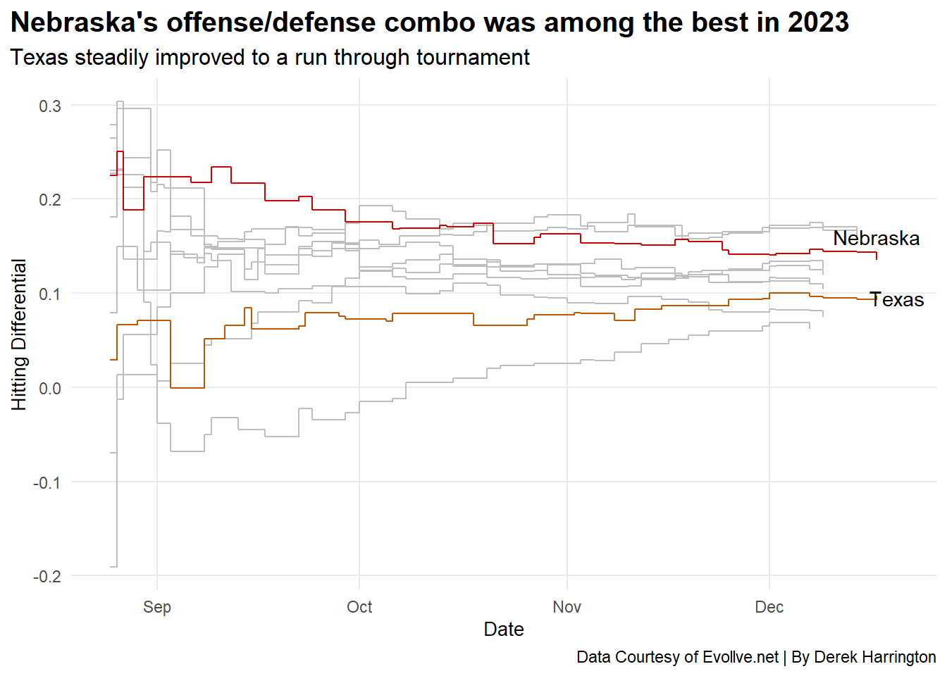
We see Nebraska once again started near the top of this statistic and continued to gradually fall, although they were still among the top three to four teams throughout the season.
Texas meanwhile, had a rough start. The Longhorns suffered some losses in the non-conference portion of their schedule and remained relatively steady through Big 12 play. Toward the second half of November and then throughout the tournament, they began climbing, meaning the offense for the Longhorns was picking up. Just in time. After the tournament ended, Nebraska still had a top 3 hitting differential among the top 10 teams, but Texas walked away with the title.
We know hitting efficiency is a stat that everyone wants to look at, especially during a game, to see how much success a team is having. While it can give an instant snapshot of a game, season, etc., it’s not the entire story. Earned points and points given away per set can show which teams are great at scoring the ball in a variety of ways, and who struggles with giving away free points.
Perhaps the best metric for analyzing and predicting a team’s success is hitting differential. While it’s not 100% foolproof (Hello Texas’ run through the 2023 tournament!), it does a decent job at predicting who the elite teams are.